![]()
![]()
This chapter describes the layers and their properties that can be used with the Neural Network Libraries.
IO
Input/output data.
Basic
Perform computatoins on artificial neurons.
(Binary layer required for binary neural networks)
Activation
Apply non-linear conversion to input data for activation.
(Binary layer required for binary neural networks)
Pooling
Perform pooling.
Parameter
Parameters to be optimized.
LoopControl
Control repetitive processes.
Unit, Math, Loss, Others, Others (Pre Process)
For various purposes, from arithmetic operations on tensor elements to preprocessing data.
Arithmetic (Scalar, 2 Inputs), Logical, Validation
For arithmetic/logical opertaions, precision computation, etc.
Common layer properties include the layer name and the properties that are automatically calculated based on the inter-layer link status and layer-specific properties.
| Name | This indicates the layer name.
Each layer name must be unique in the graph. |
| Input | This indicates the layer’s input size. |
| Output | This indicates the layer’s output size. |
| CostParameter | This indicates the number of parameters that the layer contains. |
| CostAdd | This indicates the number of multiplications required in forward calculation and the number of additions that cannot be performed during the same time. |
| CostMultiply | This indicates the number of additions required in forward calculation and the number of multiplications that cannot be performed during the same time. |
| CostMultiplyAdd | This indicates the number of multiplications and additions required in forward calculation (the number of multiplications and the number of additions that can be performed during the same time). |
| CostDivision | This indicates the number of divisions required in forward calculation. |
| CostExp | This indicates the number of exponentiation required in forward calculation. |
| CostIf | This indicates the number of conditional decisions required in forward calculation. |
This is the neural network input layer.
| Size | Specifies the input size.
For image data, the size is specified in the “the number of colors,height,width” format. For example, for a RGB color image whose width is 32 and height is 24, specify “3,24,32”. For a monochrome image whose width is 64 and height is 48, specify “1,48,64”. For CSV data, the size is specified in the “the number of rows, the number of columns” format. For example, for CSV data consisting of 16 rows and 1 column, specify “16,1”. For CSV data consisting of 12 rows and 3 columns, specify “12,3”. |
| Dataset | Specifies the name of the variable to input into this Input layer. |
| Generator | Specifies the generator to use in this input layer. If the Generator property is not set to None, the data that the generator generates is used in place of the variable specified by Dataset during optimization.
None: Data generation is not performed. Uniform: Uniform random numbers between -1.0 and 1.0 are generated. Normal: Gaussian random numbers with 0.0 mean and 1.0 variance are generated. Constant: Data whose elements are all constant (1.0) is generated. |
| GeneratorMultiplier | Specifies the multiplier to apply to the values that the generator generates. |
This is the output layer of a neural network that minimizes the squared errors between the variables and dataset variables. It is used when solving regression problems with neural networks (when optimizing neural networks that output continuous values).
| T.Dataset | Specifies the name of the variable expected to be the output of this SquaredError layer. |
| T.Generator | Specifies the generator to use in place of the dataset. If the Generator property is not set to None, the data that the generator generates is used in place of the variable specified by T.Dataset during optimization.
None: Data generation is not performed. Uniform: Uniform random numbers between -1.0 and 1.0 are generated. Normal: Gaussian random numbers with 0.0 mean and 1.0 variance are generated. Constant: Data whose elements are all constant (1.0) is generated. |
| T.GeneratorMultiplier | Specifies the multiplier to apply to the values that the generator generates. |
This is the output layer of a neural network that minimizes the Huber loss between the variables and dataset variables. Like Squared Error, this is used when solving regression problems with neural networks. Using this in place of Squared Error has the effect of stabilizing the training process.
![]()
(i indicates the difference between the dataset and inputs.)
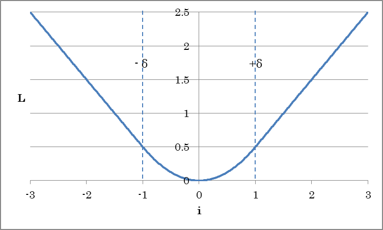
| Delta | Specify δ, which is used as a threshold for increasing the loss linearly. |
Other properties are the same as those of SquaredError.
This is the output layer of a neural network that minimizes absolute error between the variables and dataset variables. Like Squared Error, this is used when solving regression problems with neural networks. The properties are the same as those of SquaredError.
This is the output layer of a neural network that minimizes absolute error exceeding the range specified by Epsilon between the variables and dataset variables. Like Squared Error, this is used when solving regression problems with neural networks.
| Epsilon | Specify ε |
Other properties are the same as those of SquaredError.
This is the output layer of a neural network that minimizes the mutual information between the variable and dataset variables. It is used to solve binary classification problems (0 or 1). The input to BinaryCrossEntropy must be between 0.0 and 1.0 (probability), and the dataset variable must be 0 or 1. All the properties are the same as those of SquaredError.
This is the output layer of a neural network that minimizes the cross entropy between the variables and dataset variables. SigmoidCrossEntropy is equivalent to Sigmoid+BinaryCrossEntropy during training, but computing them at once has the effect of reducing computational error. The properties are the same as those of SquaredError.
Reference
If SigmoidCrossEntropy is used in place of Sigmoid+BinaryCrossEntropy, continuous values without undergoing Sigmoid processing will be output for the evaluation results.
This is the output layer of a neural network that minimizes the cross entropy between the variables and dataset variables provided by the category index. The properties are the same as those of SquaredError.
This is the output layer of a neural network that minimizes the cross entropy between the variables and dataset variables provided by the category index. SoftmaxCrossEntropy is equivalent to Softmax+CategoricalCrossEntropy during training, but computing them at once has the effect of reducing computational error. The properties are the same as those of SquaredError.
Reference
If SoftmaxCrossEntropy is used in place of Softmax+CategoricalCrossEntropy, continuous values without undergoing Softmax processing will be output for the evaluation results.
This is the output layer of a neural network that minimizes the Kullback Leibler distance between the probability distribution (p), which is a polynomial distribution input, and the dataset variable (q). The properties are the same as those of SquaredError.
This is a neural network parameter.
| Size | Specify the size of the parameter. | File | When using a pre-trained parameter, specify the file containing the parameter with an absolute path. If a file is specified and the parameter is to be loaded from a file, initialization with the initializer will be disabled. |
Initializer | Specify the initialization method for the parameter. Uniform: Initialization is performed using uniform random numbers between -1.0 and 1.0. UniformAffineGlorot: Initialization is performed by applying the multiplier recommended by Xavier Glorot to uniform random numbers. UniformConvolutionGlorot: Initialization is performed by applying the multiplier recommended by Xavier Glorot to uniform random numbers. Normal: Initialization is performed using Gaussian random numbers with 0.0 mean and 1.0 variance (default). NormalAffineHeForward: Initialization is performed by applying the multiplier recommended by Kaiming He to Gaussian random numbers (Forward Case). NormalAffineHeBackward: Initialization is performed by applying the multiplier recommended by Kaiming He to Gaussian random numbers (Backward Case). NormalAffineGlorot: Initialization is performed by applying the multiplier recommended by Xavier Glorot to Gaussian random numbers. NormalConvolutionHeForward: Initialization is performed by applying the multiplier recommended by Kaiming He to Gaussian random numbers (Forward Case). NormalConvolutionHeBackward: Initialization is performed by applying the multiplier recommended by Kaiming He to Gaussian random numbers (Backward Case). NormalConvolutionGlorot: Initialization is performed by applying the multiplier recommended by Xavier Glorot to Gaussian random numbers. Constant: All elements are initialized with a constant (1.0). |
InitializerMultiplier | Specify the multiplier to apply to the values that the initializer generates. | LRateMultiplier | Specify the multiplier to apply to the Learning Rate specified on the Config tab. This multiplier is used to update the parameter. |
Reference
A parameter defined with the Parameter layer can be used by connecting to the W and b side connectors of Affine or Convolution or in other similar ways.
This is a buffer for temporarily storing computation results. Data input in WorkingMemory is stored in WorkingMemory. Data stored in WorkingMemory can be retrieved from the output of WorkingMemory with the same name placed in another network.
| Size | Specify the size of the buffer. | File | To specify the content of the buffer in advance, specify the file containing the data with an absolute path. If a file is specified and the data is to be loaded from a file, initialization with the initializer will be disabled. |
Initializer | Specify the initialization method for the parameter. Uniform: Initialization is performed using uniform random numbers between -1.0 and 1.0. Normal: Initialization is performed using Gaussian random numbers with 0.0 mean and 1.0 variance (default). Constant: All elements are initialized with a constant (1.0). |
InitializerMultiplier | Specify the multiplier to apply to the values that the initializer generates. |
The affine layer is a fully-connected layer that has connections from all inputs to all output neurons specified with the OutShape property.
o = Wi+b
(where i is the input, o is the output, W is the weight, and b is the bias term.)
| OutShape | Specifies the number of output neurons of the Affine layer. |
| WithBias | Specifies whether to include a bias term (b). |
| ParameterScope | Specifies the name of the parameter used by this layer.
The parameter is shared between layers with the same ParameterScope. |
| W.File | When using pre-trained weight W, specifies the file containing W with an absolute path.
If a file is specified and weight W is to be loaded from a file, initialization with the initializer will be disabled. |
| W.Initializer | Specifies the initialization method for weight W.
Uniform: Initialization is performed using uniform random numbers between -1.0 and 1.0. UniformAffineGlorot: Initialization is performed by applying the multiplier recommended by Xavier Glorot to uniform random numbers. Normal: Initialization is performed using Gaussian random numbers with 0.0 mean and 1.0 variance. NormalAffineHeForward: Initialization is performed by applying the multiplier recommended by Kaiming He to Gaussian random numbers (Forward Case). NormalAffineHeBackward: Initialization is performed by applying the multiplier recommended by Kaiming He to Gaussian random numbers (Backward Case). NormalAffineGlorot: Initialization is performed by applying the multiplier recommended by Xavier Glorot to Gaussian random numbers (default). Constant: All elements are initialized with a constant (1.0). |
| W.InitializerMultiplier | Specifies the multiplier to apply to the values that the initializer generates. |
| W.LRateMultiplier | Specifies the multiplier to apply to the Learning Rate specified on the CONFIG tab. This multiplier is used to update weight W.
For example, if the Learning Rate specified on the CONFIG tab is 0.01 and W.LRateMultiplier is set to 2, weight W will be updated using a Learning Rate of 0.02. |
| b.* | This is used to set the bias b. The properties are the same as those of W. |
The convolution layer is used to convolve the input.
Ox,m = Σ_i,n Wi,n,m Ix+i,n + bm (one-dimensional convolution)
Ox,y,m = Σ_i,j,n Wi,j,n,m Ix+i,y+j,n + bm (two-dimensional convolution)
(where O is the output; I is the input; i,j is the kernel size; x,y,n is the input index; m is the output map (OutMaps property), W is the kernel weight, and b is the bias term of each kernel)
| KernelShape | Specifies the convolution kernel size.
For example, to convolve an image with a 3 (height) by 5 (width) two-dimensional kernel, specify “3,5”. For example, to convolve a one-dimensional time series signal with a 7-tap filter, specify “7”. |
| WithBias | Specifies whether to include the bias term (b). |
| OutMaps | Specifies the number of convolution kernels (which is equal to the number of output data samples).
For example, to convolve an input with 16 types of filters, specify “16”. |
| BorderMode | Specifies the type of convolution border.
valid: Convolution is performed within the border of the kernel shape for the input data size of each axis. In this case, the size of each axis of the output data is equal to input size – kernel shape + 1. full: Convolution is performed within the border even with a single sample for the input data of each axis. Insufficient data (kernel shape – 1 to the top, bottom, left, and right) within the border are padded with zeros. In this case, the size of each axis of the output data is equal to input size + kernel shape – 1. same: Convolution is performed within a border that would make the input data size the same as the output data size. Insufficient data (kernel shape/2 – 1 to the top, bottom, left, and right) within the border are padded with zeros. |
| Padding | Specifies the size of zero padding to add to the ends of the arrays before the convolution process. For example, to insert 3 pixels vertically and 2 pixels horizontally, specify “3,2”.
* ConvolutionPaddingSize: A value calculated from BorderMode is used for Padding. |
| Strides | Specifies the period of performing the convolution (after how many samples kernel convolution is performed)
The output size of an axis with Stride set to a value other than 1 will be downsampled by the specified value. For example, to convolve every two samples in the X-axis direction and every three samples in the Y-axis direction, specify “3,2”. |
| Dilation | Specifies the factor by which the kernel is to be dilated using a stride value in unit of kernel size. For example, to dilate a 3 (height) by 5 (width) two-dimensional kernel to three times the height and two times the width and perform convolution on a 7 by 9 area, specify “3,2”. |
| Group | Specifies the unit for grouping OutMaps. |
| ParameterScope | Specifies the name of the parameter used by this layer.
The parameter is shared between layers with the same ParameterScope. |
| W.File | When using pre-trained weight W, specify the file containing W with an absolute path.
If a file is specified and weight W is to be loaded from a file, initialization with the initializer will be disabled. |
| W.Initializer | Specifies the initialization method for weight W.
Uniform: Initialization is performed using uniform random numbers between -1.0 and 1.0. UniformConvolutionGlorot: Initialization is performed by applying the multiplier recommended by Xavier Glorot to uniform random numbers. Normal: Initialization is performed using Gaussian random numbers with 0.0 mean and 1.0 variance. NormalConvolutionHeForward: Initialization is performed by applying the multiplier recommended by Kaiming He to Gaussian random numbers (Forward Case). NormalConvolutionHeBackward: Initialization is performed by applying the multiplier recommended by Kaiming He to Gaussian random numbers (Backward Case). NormalConvolutionGlorot: Initialization is performed by applying the multiplier recommended by Xavier Glorot to Gaussian random numbers (default). Constant: All elements are initialized with a constant (1.0). |
| W.InitializerMultiplier | Specifies the multiplier to apply to the values that the initializer generates. |
| W.LRateMultiplier | Specify the multiplier to apply to the Learning Rate specified on the CONFIG tab. This multiplier is used to update weight W.
For example, if the Learning Rate specified on the CONFIG tab is 0.01 and W.LRateMultiplier is set to 2, weight W will be updated using a Learning Rate of 0.02. |
| b.* | This is used to set the bias b. The properties are the same as those of W. |
The convolution layer is used to convolve the input for each map. The operation of DepthwiseConvolution is equivalent to setting Group of a convolution whose number of input and output maps is the same to OutMaps.
Ox,y,n = Σ_i,j Wi,j Ix+i,y+j,n + bn (two-dimensional convolution, when Multiplier=1)
(where O is the output; I is the input; i,j is the kernel size; x,y,n is the input index; W is the kernel weight, and b is the bias term of each kernel)
| KernelShape | Specifies the convolution kernel size.
For example, to convolve an image with a 3 (height) by 5 (width) two-dimensional kernel, specify “3,5”. For example, to convolve a one-dimensional time series signal with a 7-tap filter, specify “7”. |
| WithBias | Specifies whether to include the bias term (b). |
| BorderMode | Specifies the type of convolution border.
valid: Convolution is performed within the border of the kernel shape for the input data size of each axis. In this case, the size of each axis of the output data is equal to input size – kernel shape + 1. full: Convolution is performed within the border even with a single sample for the input data of each axis. Insufficient data (kernel shape – 1 to the top, bottom, left, and right) within the border are padded with zeros. In this case, the size of each axis of the output data is equal to input size + kernel shape – 1. same: Convolution is performed within a border that would make the input data size the same as the output data size. Insufficient data (kernel shape/2 – 1 to the top, bottom, left, and right) within the border are padded with zeros. |
| Padding | Specifies the size of zero padding to add to the ends of the arrays before the convolution process. For example, to insert 3 pixels vertically and 2 pixels horizontally, specify “3,2”.
* ConvolutionPaddingSize: A value calculated from BorderMode is used for Padding. |
| Strides | Specifies the period of performing the convolution (after how many samples kernel convolution is performed)
The output size of an axis with Stride set to a value other than 1 will be downsampled by the specified value. For example, to convolve every two samples in the X-axis direction and every three samples in the Y-axis direction, specify “3,2”. |
| Dilation | Specifies the factor by which the kernel is to be dilated using a stride value in unit of kernel size. For example, to dilate a 3 (height) by 5 (width) two-dimensional kernel to three times the height and two times the width and perform convolution on a 7 by 9 area, specify “3,2”. |
| Multiplier | Specify the magnification of the number of output images relative to the number of input images. |
| ParameterScope | Specifies the name of the parameter used by this layer.
The parameter is shared between layers with the same ParameterScope. |
| W.File | When using pre-trained weight W, specify the file containing W with an absolute path.
If a file is specified and weight W is to be loaded from a file, initialization with the initializer will be disabled. |
| W.Initializer | Specifies the initialization method for weight W.
Uniform: Initialization is performed using uniform random numbers between -1.0 and 1.0. UniformConvolutionGlorot: Initialization is performed by applying the multiplier recommended by Xavier Glorot to uniform random numbers. Normal: Initialization is performed using Gaussian random numbers with 0.0 mean and 1.0 variance. NormalConvolutionHeForward: Initialization is performed by applying the multiplier recommended by Kaiming He to Gaussian random numbers (Forward Case). NormalConvolutionHeBackward: Initialization is performed by applying the multiplier recommended by Kaiming He to Gaussian random numbers (Backward Case). NormalConvolutionGlorot: Initialization is performed by applying the multiplier recommended by Xavier Glorot to Gaussian random numbers (default). Constant: All elements are initialized with a constant (1.0). |
| W.InitializerMultiplier | Specifies the multiplier to apply to the values that the initializer generates. |
| W.LRateMultiplier | Specify the multiplier to apply to the Learning Rate specified on the CONFIG tab. This multiplier is used to update weight W.
For example, if the Learning Rate specified on the CONFIG tab is 0.01 and W.LRateMultiplier is set to 2, weight W will be updated using a Learning Rate of 0.02. |
| b.* | This is used to set the bias b. The properties are the same as those of W. |
The deconvolution layer is used to deconvolve the input. The properties of deconvolution are the same as those of convolution.
The DepthwiseDeconvolution layer is used to deconvolve the input for each map. The operation of DepthwiseDeconvolution is equivalent to that of deconvolution whose Group value is the same as the number of input maps and OutMaps.
Inputs are assumed to be discrete symbols represented by integers ranging from 0 to N-1 (where N is the number of classes), and arrays of a specified size are assigned to each symbol. For example, this is used when the inputs are word indexes, and each word is converted into vectors in the beginning of a network. The output size is equal to input size × array size.
| NumClass | Specifies the number of classes N. |
| Shape | Specifies the size of the array assigned to a single symbol. |
| ParameterScope | Specifies the name of the parameter used by this layer.
The parameter is shared between layers with the same ParameterScope. |
| W.File | When using pre-trained weight W, specify the file containing W with an absolute path.
If a file is specified and weight W is to be loaded from a file, initialization with the initializer will be disabled. |
| W.Initializer | Specifies the initialization method for weight W.
Uniform: Initialization is performed using uniform random numbers between -1.0 and 1.0. Normal: Initialization is performed using Gaussian random numbers with 0.0 mean and 1.0 variance. Constant: All elements are initialized with a constant (1.0). |
| W.InitializerMultiplier | Specifies the multiplier to apply to the values that the initializer generates. |
| W.LRateMultiplier | Specifies the multiplier to apply to the Learning Rate specified on the CONFIG tab. This multiplier is used to update weight W.
For example, if the Learning Rate specified on the CONFIG tab is 0.01 and W.LRateMultiplier is set to 2, weight W will be updated using a Learning Rate of 0.02. |
MaxPooling outputs the maximum value of local inputs.
| KernelShape | Specifies the size of the local region for sampling the maximum value.
For example, to output the maximum value over a 3 (height) by 5 (width) region, specify “3,5”. |
| Strides | Specifies the period for sampling maximum values (after how many samples maximum values are determined)
The output size of each axis will be downsampled by the specified value. For example, to sample maximum values every two samples in the X-axis direction and every three samples in the Y-axis direction, specify “3,2”. * Use the same value as KernelShape for KernelShape:Strides. |
| IgnoreBorder | Specifies the border processing method.
True: Processing is performed over regions that have enough samples to fill KernelShape. Samples near the border where there are not enough samples to fill KernelShape are ignored. False: Samples near the border are not discarded. Processing is performed even over regions that only have one sample. |
| Padding | Specifies the size of zero padding to add to the ends of the arrays before the pooling process.
For example, to add two pixels of zero padding to the top and bottom and one pixel of zero padding to the left and right of an image, specify “2,1”. |
AveragePooling outputs the average of local inputs. The properties are the same as those of MaxPooling.
GlobalAveragePooling outputs the average of the entire last two dimensions of an array. GlobalAveragePooling is equivalent to AveragePooling with PoolShape and Strides set to the number of samples in the last two dimensions of the input array.
SumPooling outputs the sum of local inputs. The properties are the same as those of MaxPooling.
Unpooling copies a single input to multiple inputs in order to generate data larger in size than the input data.
| KernelShape | Specify the size of data to copy.
For example, if you want to copy a data sample twice in the vertical direction and three times in the horizontal direction (output data whose size is twice as large in the vertical direction and three times as large in the horizontal direction), specify “2,3”. |
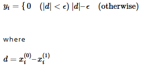
Tanh outputs the result of taking the hyperbolic tangent of the input.
o=tanh(i)
(where o is the output and i is the input)
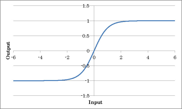
HardTanh outputs -1 for inputs less than or equal to -1, +1 for inputs greater than equal to +1, and the input value for inputs that are between -1 and +1. This is an activation function that approximates using a lighter computation method than Tanh.
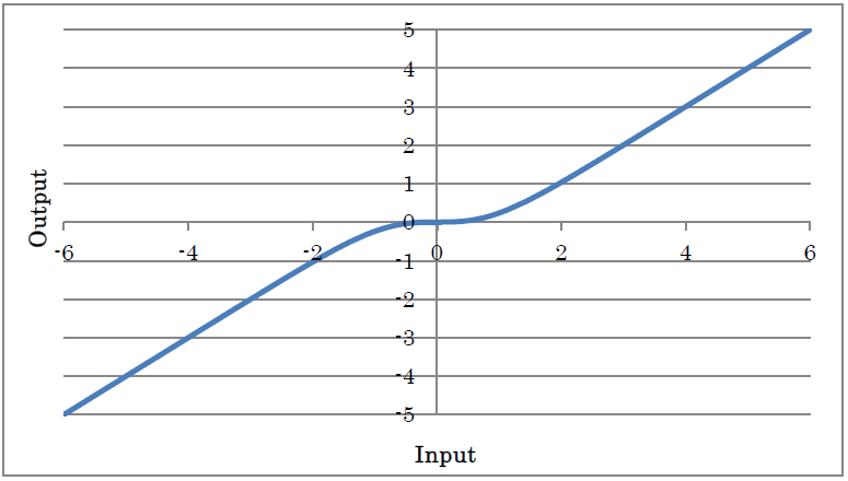
TanhShrink outputs the result of applying TanhShrink to the input.
y=x – tanh(x)
(where y is the output and x is the input)
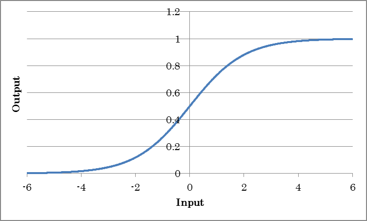
Sigmoid outputs the result of taking the sigmoid of the input. This is used when you want to obtain probabilities or output values ranging from 0.0 to 1.0.
o=sigmoid(i)
(where o is the output and i is the input)
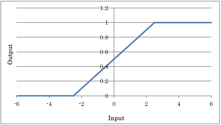
HardTanh outputs -0 for inputs less than or equal to -2.5, +1 for inputs greater than or equal to +2.5, and input value×0.2+0.5 for inputs that are between -2.5 and +2.5. It is an activation function that approximates using a lighter computation method than Sigmoid.
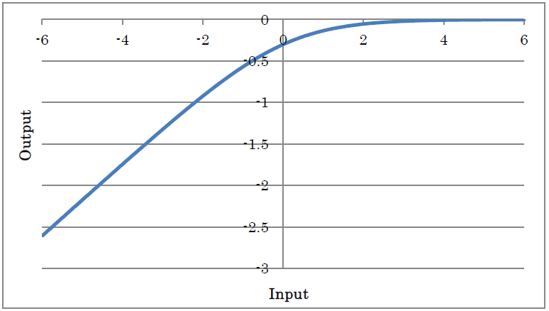
LogSigmoid outputs the result of applying LogSigmoid to the input.
y=log(1/(1+exp(-x)))
(where y is the output and x is the input)
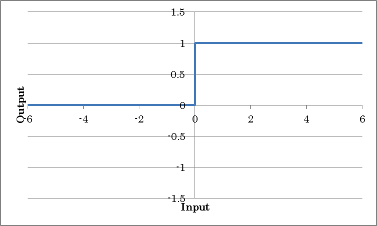
ReLU outputs the result of applying the rectified linear unit (ReLU) to the input.
o=max(0, i)
(where o is the output and i is the input)
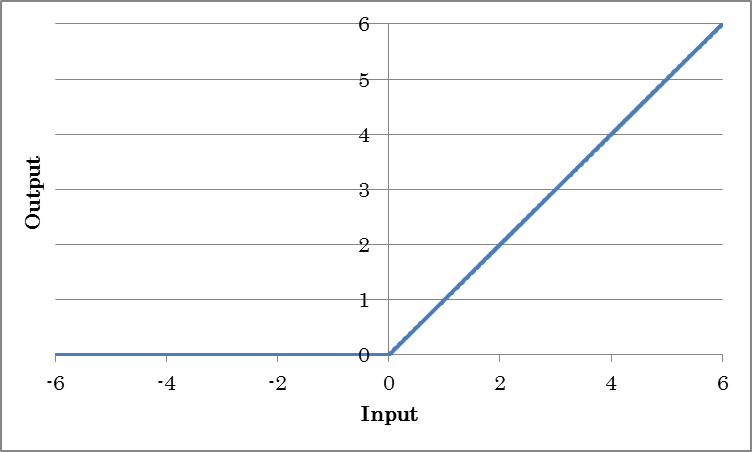
| InPlace | If set to True, the memory needed for training is conserved by sharing the input and output buffers. To apply InPlace automatically when it is possible, specify *AutoInPlaceOnce. |
Concatenated ReLU (CReLU) applies Relu to each of the negated input signals, concatenates each result on the axis indicated by the Axis property, and outputs the final result.
Unlike ReLU, which always outputs 0 for inputs less than 0, LeakyReLU multiplies inputs less than 0 with a constant value to output results.
o=max(0, i) + a min(0, i)
(where o is the output and i is the input)
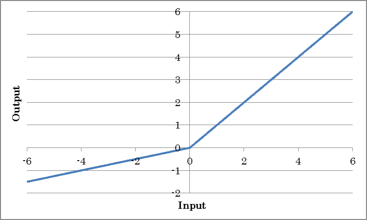
| alpha | Specify negative gradient a. | InPlace | If set to True, the memory needed for training is conserved by sharing the input and output buffers. To apply InPlace automatically when it is possible, specify *AutoInPlaceOnce. |
Unlike ReLU, which always outputs 0 for inputs less than 0, parametric ReLU (PReLU) multiplies inputs less than 0 with a constant value to output results. The value of a, which is a gradient less than 0, is obtained from training.
o=max(0, i) + a min(0, i)
(where o is the output and i is the input)
| BaseAxis | Of the available inputs, specifies the index (that starts at 0) of the axis that individual a’s are to be trained on. For example, for inputs 4,3,5, to train individual a’s for the first dimension (four elements), set BaseAxis to 0. |
| ParameterScope | Specifies the name of the parameter used by this layer.
The parameter is shared between layers with the same ParameterScope. |
| slope.File | When using pre-trained gradient a, specifies the file containing a with an absolute path.
If a file is specified and weight slope is to be loaded from a file, initialization with the initializer will be disabled. |
| slope.Initializer | Specifies the initialization method for gradient a.
Uniform: Initialization is performed using uniform random numbers between -1.0 and 1.0. Normal: Initialization is performed using Gaussian random numbers with 0.0 mean and 1.0 variance. Constant: All elements are initialized with a constant (1.0). |
| slope.InitializerMultiplier | Specifies the multiplier to apply to the values that the initializer generates. |
| slope.LRateMultiplier | Specifies the multiplier to apply to the Learning Rate specified on the CONFIG tab. This multiplier is used to update gradient a.
For example, if the Learning Rate specified on the CONFIG tab is 0.01 and slope.LRateMultiplier is set to 2, gradient a will be updated using a Learning Rate of 0.02. |
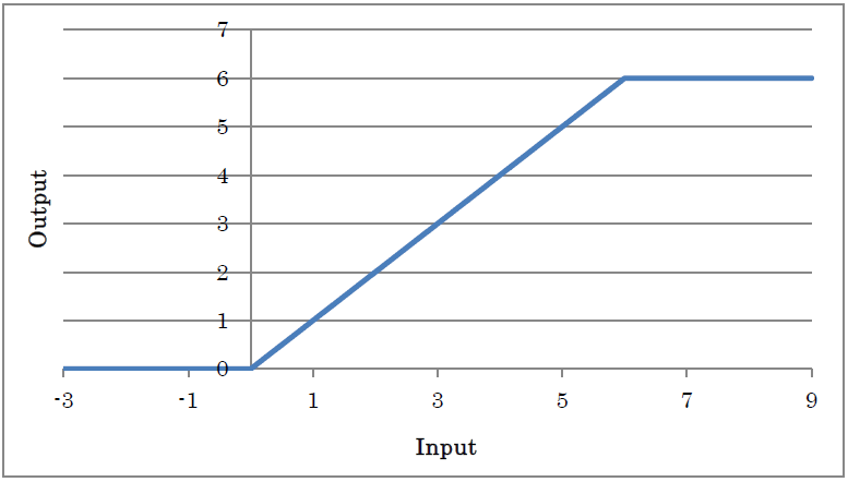
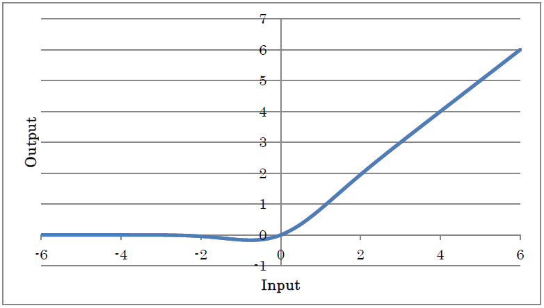
ReLU6 outputs the result of applying ReLU to the input with the maximum output value limited to 6.
y=min(max(0,x),6)
(where y is the output and x is the input)
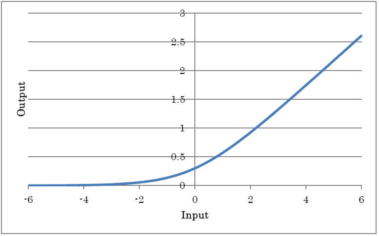
ELU outputs the result of applying the exponential linear unit (ELU) to the input.
o=max(0, i) + alpha(exp(min(0, i)) – 1)
(where o is the output and i is the input)
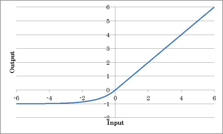
| Alpha | Specify coefficient alpha for negative outputs. |
Concatenated ELU (CELU) applies ELU to each of the negated input signals, concatenates each result on the axis indicated by the Axis property, and outputs the final result.
SELU outputs the result of applying the scaled exponential linear unit (SELU) to the input.
o=lambda {max(0, i) + alpha(exp(min(0, i)) – 1)}
(where o is the output and i is the input)
| Scale | Specify the whole scale lambda. |
| Alpha | Specify coefficient alpha for negative outputs. |
GELU outputs the result of applying the Gaussian error unit (GELU) to the input.
y=xP(X≤x)=xΦ(x)
y=0.5x(1+tanh((√2/π)(x+0.044715 x3)))
(where y is the output and x is the input)
Softplus outputs the result of applying Softplust to the input.
y=log(1+exp(x))
(where y is the output and x is the input)
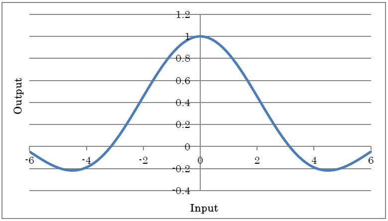
y=sin(x)/x (x != 0)
y=1 (x==0)
(where y is the output and x is the input)
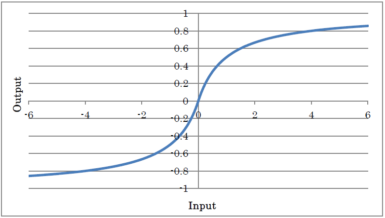
SoftSign outputs the result of applying SoftSign to the input.
y=x/(1+|x|)
(where y is the output and x is the input)
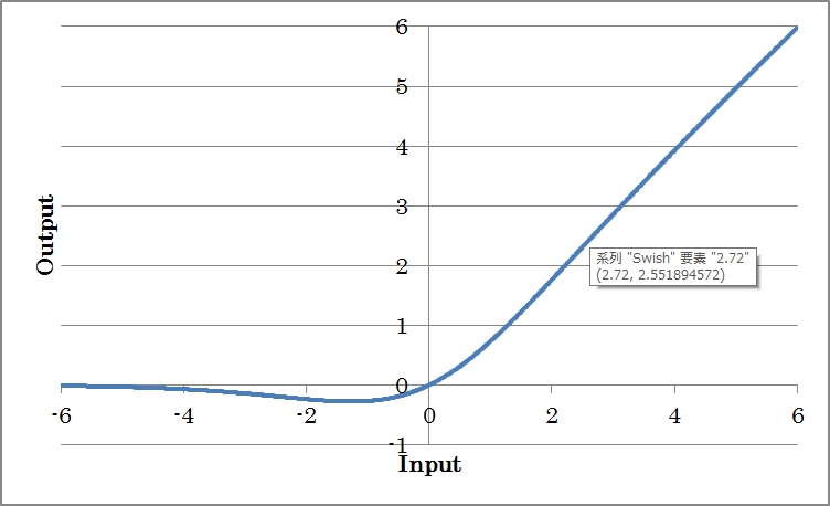
Swish outputs the result of taking the swish of the input.
o=i/(1+exp(-i))
(where o is the output and i is the input)
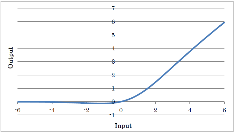
Mish outputs the result of taking the mish of the input.
y=x tanh(log(1+exp(x))
(where y is the output and x is the input)
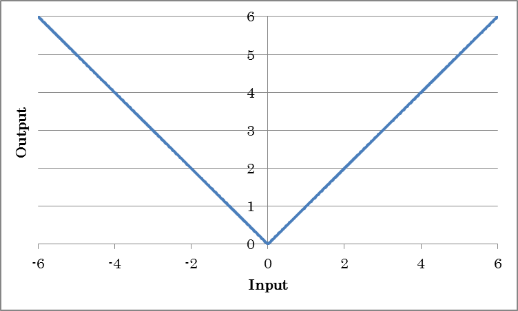
Abs outputs the absolute values of inputs.
o=abs(i)
(where o is the output and i is the input)
Softmax outputs the Softmax of inputs. This is used when you want to obtain probabilities in a categorization problem or output values ranging from 0.0 to 1.0 that sum up to 1.0.
ox=exp(ix) / Σ_jexp(ij)
(where o is the output, i is the input, and x is the data index)
The Loop Control layer is useful for configuring networks with a loop structure, such as residual networks and recurrent neural networks.
RepeatStart is a layer that indicates the start position of a loop. Layers placed between RepeatStart and RepeatEnd are created repeatedly for the number of times specified by the Times property of Repeat Start.
Notes
The array sizes of the layers between RepeatStart and RepeatEnd must be the same. Structures whose array sizes differ between repetitions cannot be written.
RepeatEnd is a layer that indicates the end position of a loop.
RecurrentInput is a layer that indicates the time loop start position of a recurrent neural network. The axis specified by the Axis property is handled as the time axis. The length of a time loop is defined by the number of elements specified by the Axis property of the input data.
RecurrentOutput is a layer that indicates the time loop end position of a recurrent neural network.
Delay is a layer that indicates the time delay signal in a recurrent neural network.
| Size | Specifies the size of the time delay signal. |
| Initial.Dataset | Specifies the name of the variable to be used as the initial value of the time delay signal. |
| Initial.Generator | Specifies the generator to use in place of the dataset. If the Generator property is not set to None, the data that the generator generates is used in place of the variable specified by T.Dataset during optimization.
None: Data generation is not performed. Uniform: Uniform random numbers between -1.0 and 1.0 are generated. Normal: Gaussian random numbers with 0.0 mean and 1.0 variance are generated. Constant: Data whose elements are all constant (1.0) is generated. |
| Initial.GeneratorMultiplier | Specifies the multiplier to apply to the values that the generator generates. |
The quantization layer is used to quantize weights and data.
FixedPointQuantize performs linear quantization.
| Sign | Specify whether to include signs.
When set to false, all values after quantization will be positive. |
| N | Specify the number of quantization bits. |
| Delta | Specify the quantization step size. |
| STEFineGrained | Specify the gradient calculation method for backward processing.
True: The gradient is always 1. False: The gradient is 1 between the maximum and minimum values of the range that can be expressed through quantization; otherwise it is 0. |
Pow2Quantize performs power-of-two quantization.
| Sign | Specify whether to include signs.
When set to false, all values after quantization will be positive. |
| WithZero | Specify whether to include zeros.
When set to false, values after quantization will not include zeros. |
| N | Specify the number of quantization bits. |
| M | Specify the maximum value after quantization as 2^M. |
| STEFineGrained | Specify the gradient calculation method for backward processing.
True: The gradient is always 1. False: The gradient is 1 between the maximum and minimum values of the range that can be expressed through quantization; otherwise it is 0. |
BinaryConnectAffine is an Affine layer that uses W, which has been converted into the binary values of -1 and +1.
o = sign(W)i+b
(where i is the input, o is the output, W is the weight, and b is the bias term.)
| Wb.* | Specifies the weight Wb settings to use after the conversion into binary values. The properties are the same as those of W for the Affine layer. |
For details on other properties, see the Affine layer.
BinaryConnectConvolution is a convolution layer that uses W, which has been converted into the binary values of -1 and +1.
Ox,y,m = Σ_i,j,n sign(Wi,j,n,m) Ix+i,y+j,n + bm (two-dimensional convolution)
(where O is the output; I is the input; i,j is the kernel size; x,y,n is the input index; m is the output map (OutMaps property), W is the kernel weight, and b is the bias term of each kernel)
| Wb.* | Specifies the weight Wb settings to use after the conversion into binary values. The properties are the same as those of W for the Convolution layer. |
For details on other properties, see the Convolution layer.
BinaryWeightAffine is an affine layer that uses W, which has been converted into binary values of -1 and +1, and then scaled in order to make the output closer to the normal Affine layer.
o = a sign(W)i +b
(where i is the input, o is the output, W is the weight, a is the scale, and b is the bias term.)
BinaryWeightConvolution is an affine layer that uses W, which has been converted into binary values of -1 and +1, and then scaled to make the output closer to the normal Convolution layer.
Ox,y,m = Σ_i,j,n sign(Wi,j,n,m) Ix+i,y+j,n * a+ bm (two-dimensional convolution)
(where O is the output; I is the input; i,j is the kernel size; x,y,n is the input index; m is the output map (OutMaps property), W is the kernel weight, a is the scale, and b is the bias term of each kernel)
Binarytanh outputs -1 for inputs less than or equal to 0 and +1 for inputs great than 0.
BinarySigmoid outputs 0 for inputs less than or equal to 0 and +1 for inputs great than 0.
The unit layer provides a function for inserting other networks in the middle of a network. By using the unit layer, you can insert a collection of layers defined as a network in the middle of another network.
A network that another network is inserted into using the unit layer is called a caller network, and the network to be inserted into another network using the unit layer is called a unit network.
Inserts a unit network into the current caller network.
| Network | Specify the name of the unit network to be inserted. |
| ParameterScope | Specify the name of the parameter used by this unit.
The parameter is shared between units with the same ParameterScope. |
| (Other properties) | Specify the properties of the unit network to be inserted. |
Set the parameters of the unit network to allow editing as unit properties from the caller network. You can specify the name of an argument layer for the other layer properties in the unit network to use the argument layer values from the other layers in the unit network. The implemented argument layer values can be specified through the unit properties implemented in the caller network.
| Value | Specify the default parameter value. |
| Type | Specify the parameter type.
Boolean: True or False Int: Integer IntArray: Array of integers PInt: Integer greater than equal to 1 PIntArray: Array of integers greater than equal to 1 PIntArrays: Array of array of integers greater than equal to 1 UInt: Unsigned integer UIntArray: Array of unsigned integers Float: Floating-point number FloatArray: Array of floating-point numbers FloatArrays: Array of array of floating-point numbers Text: Character string File: File name |
| Search | Specify for the caller network whether to include the parameter in the automatic structure search. |
Performs a Fourier transform of the complex input and complex output. The last dimension of the input array must be complex (real part and imaginary part).
| SignalNDim | Specify the number of dimensions of the signal to perform the Fourier transform of. For example, specify 1 for a one-dimensional Fourier transform and 2 for a two-dimensional Fourier transform. |
| Normalized | Scales the Fourier transform result by a constant factor indicated by the following formula and exports the final result. |
Performs an inverse Fourier transform of the complex input and complex output.
| SignalNDim | Specify the number of dimensions of the signal to perform the inverse Fourier transform of. For example, specify 1 for a one-dimensional inverse Fourier transform and 2 for a two-dimensional inverse Fourier transform. |
| Normalized | Specify the constant to multiply the inverse Fourier transform result by.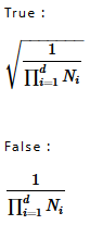 |
LSTM unit is an experimentally implemented unit. For now, we recommend that you write the structure of LSTM directly instead of using LSTM unit.
Reference:tutorial.recurrent_neural_networks.long_short_term_memory(LSTM)
Sum determines the sum of the values of the specified dimension.
| Axis | Specifies the index (starting at 0) of the axis to sum the values of. |
| KeepDims | Specifies whether to hold the axis whose values have been summed. |
Mean determines the average of the values of the specified dimension.
| Axis | Specifies the index (starting at 0) of the axis whose values will be averaged |
| KeepDims | Specifies whether to hold the axis whose values have been averaged. |
Prod determines the product of the values of the specified dimension.
| Axis | Specifies the index (starting at 0) of the axis to multiply the values of. |
| KeepDims | Specifies whether to hold the axis whose values have been multiplied. |
Max determines the maximum of the values of the specified dimension.
| Axis | Specifies the index (starting at 0) of the axis on which to determine the maximum value. |
| KeepDims | Specifies whether to hold the axis whose maximum value has been determined. |
| OnlyIndex | Specify the Max output type. True: The index with the maximum value is output. False: The maximum value is output. |
Min determines the minimum of the values of the specified dimension.
| Axis | Specifies the index (starting at 0) of the axis on which to determine the minimum value. |
| KeepDims | Specifies whether to hold the axis whose minimum value has been determined. | OnlyIndex | Specify the Min output type. True: The index with the minimum value is output. False: The minimum value is output. |
Log calculates the natural logarithm with base e.
Exp calculates the exponential function with base e.
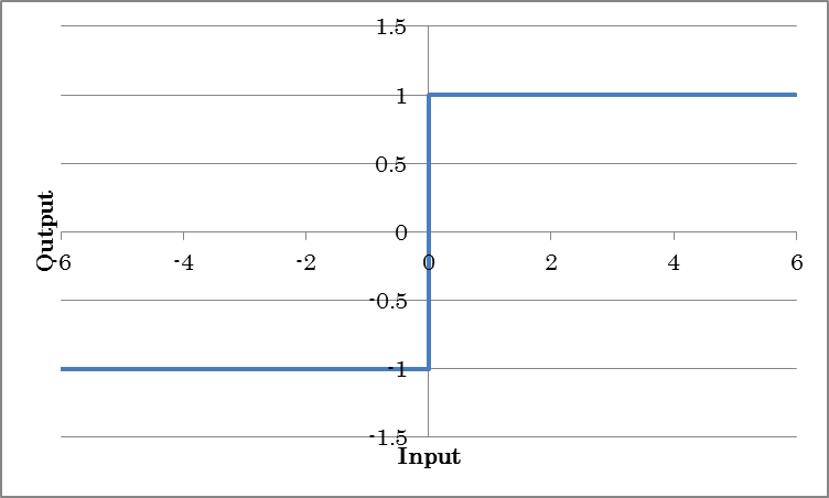
Sign outputs -1 for negative inputs, +1 for positive inputs, and alpha for 0.
| Alpha | Specifies the output corresponding to input 0. |
Reference
When compared to BinaryTanh, the operation is similar to forward computation (except for the behavior when the input is 0), but the operation of backward computation is completely different. Unlike BinaryTanh, which sets the derivative to 0 when the absolute value of the input data is 1 or greater, Sign passes through the back propagation derivative as its own derivative.
BatchMatmul calculates the matrix multiplication of the matrix expressed by the last two dimensions of input (A) and connector R input (B). If matrix A is L×N and matrix B is N×M, the output matrix will be L×M.
BatchInv outputs the inverse matrix of the last two dimensions of the input.
Round rounds the input value.
Ceil rounds up the fraction of the input value.
Floor truncates the fraction of the input value.
The trigonometric layer calculates the trigonometric function of each element.
| Layer name | Expression |
| Sin | o=sin(i) |
| Cos | o=cos(i) |
| Tan | o=tan(i) |
| Sinh | o=sinh(i) |
| Cosh | o=cosh(i) |
| ASin | o=arcsin(i) |
| ACos | o=arccos(i) |
| ATan | o=arctan(i) |
| ASinh | o=asinh(i) |
| ACosh | o=asinh(i) |
| ATanh | o=atanh(i) |
(where i is the input and o is the output)
Various arithmetic operations can be performed on each element using a real number specified by the Value property.
| Layer name | Expression |
| AddScalar | o=i+value |
| MulScalar | o=i*value |
| RSubScalar | o=value-i |
| RDivScalar | o=value/i |
| PowScalar | o=i value |
| RPowScalar | o=value i |
| MaximumScalar | o=max (i,value) |
| MinimumScalar | o=min(i,value) |
(where i is the input, o is the output, and value is the real number)
Various arithmetic operations can be performed on each element using two inputs.
| Layer | Expression |
| Add2 | o=i1+i2 |
| Sub2 | o=i1-i2 |
| Mul2 | o=i1*i2 |
| Div2 | o=i1/i2
Connect the input for i2 in the right hand side to connector R. |
| Pow2 | o=i1i2
Connect the input for i2 in the right hand side to connector R. |
| Maxmum2 | o=max(i1,i2) |
| Minimum2 | o=min(i1,i2) |
(where i1 and i2 are inputs and o is the output)
Various arithmetic operations are performed on each element using at least two inputs.
| Layer | Expression |
| AddN | y=Σxi |
| MulN | y=Πxi |
(where i1 and i2 are inputs and o is the output)
Various logical operations can be performed on each element using two inputs or one input and a value specified by the Value property. The logical operation output is 0 or 1.
| Layer name | Process |
| LogicalAnd | o= i1 and i2 |
| LogicalOr | o= i1 or i2 |
| LogicalXor | o= i1 xor i2 |
| Equal | o= i1 == i2 |
| NotEqual | o= i1 != i2 |
| GreaterEqual | o= i1 >= i2 |
| Greater | o= i1 > i2 |
| LessEqual | o= i1 <= i2 |
| Less | o= i1 < i2 |
| LogicalAndScalar | o= i and value |
| LogicalOrScalar | o= i or value |
| LogicalXorScalar | o= i xor value |
| EqualScalar | o= i == value |
| NotEqualScalar | o= i != value |
| GreaterEqualScalar | o= i >= value |
| GreaterScalar | o= i > value |
| LessEqualScalar | o= i <= value |
| LessScalar | o= i < value |
| LogicalNot | o= !i |
Notes
A logical operation layer does not support back propagation.
The input data and variable T in the dataset indicating correct values are converted into binary values (0 or 1) depending on whether the values are greater than or equal to 0.5. Then, each unmatched data sample is evaluated. If the input data match the correct binary value, 0 is output. Otherwise, 1 is output.
| T.Dataset | Specifies the name of the variable expected to be the output of this layer. |
| T.Generator | Specifies the generator to use in place of the dataset. If the Generator property is not set to None, the data that the generator generates is used in place of the variable specified by T.Dataset during optimization.
None: Data generation is not performed. Uniform: Uniform random numbers between -1.0 and 1.0 are generated. Normal: Gaussian random numbers with 0.0 mean and 1.0 variance are generated. Constant: Data whose elements are all constant (1.0) is generated. |
| T.GeneratorMultiplier | Specifies the multiplier to apply to the values that the generator generates. |
Based on the input data indicating the probability or score of each category and variable T in the dataset indicating the category index, each data sample is evaluated as to whether the probability or score of the correct category is within the top N of all categories. If the probability or score of the correct category is within the top N, 0 is output. Otherwise, 1 is output.
| Axis | Specifies the index of the axis indicating the category. |
| N | Specifies the lowest ranking N that will be considered correct.
For example, if you want to allow only the maximum probability or score of the correct category to be considered correct, specify 1. If you want to allow only the top five probabilities or scores of the correct category to be considered correct, specify 5. |
| T.Dataset | Specifies the name of the variable expected to be the output of this layer. |
| T.Generator | Specifies the generator to use in place of the dataset. If the Generator property is not set to None, the data that the generator generates is used in place of the variable specified by T.Dataset during optimization.
None: Data generation is not performed. Uniform: Uniform random numbers between -1.0 and 1.0 are generated. Normal: Gaussian random numbers with 0.0 mean and 1.0 variance are generated. Constant: Data whose elements are all constant (1.0) is generated. |
| T.GeneratorMultiplier | Specifies the multiplier to apply to the values that the generator generates. |
The input is normalized to 0 mean and 1 variance. Inserting this layer after Convolution or Affine has the effect of improving accuracy and accelerating convergence.
ox=(ix-meani) *gammax/sigmax +betax
(where o is the output, i is the input, and x is the data index)
| Axes | Of the available inputs, specifies the index (that starts at 0) of the axis to be normalized individually. For example, for inputs 4,3,5, to individually normalize the first dimension (four elements), set Axis to 0. To individually normalize the second and third dimensions (elements 3,5), set Axes to 1,2. |
| DecayRate | Specifies the decay rate (0.0 to 1.0) to apply when updating the mean and standard deviation of the input data during training. The closer the value is to 1.0, the more the mean and standard deviation determined from past data are retained. |
| Epsilon | Specifies the value to add to the denominator (standard deviation of the input data) to prevent division by zero during normalization. |
| BatchStat | Specifies whether to use the average variance calculated for each mini-batch in batch normalization.
True: The average variance calculated for each mini-batch is used. |
| ParameterScope | Specifies the name of the parameter used by this layer.
The parameter is shared between layers with the same ParameterScope. |
| beta.File | When using pre-trained beta, specifies the file containing beta with an absolute path.
If a beta is specified and is to be loaded from a file, initialization with the initializer will be disabled. |
| beta.Initializer | Specifies the initialization method for beta.
Uniform: Initialization is performed using uniform random numbers between -1.0 and 1.0. Normal: Initialization is performed using Gaussian random numbers with 0.0 mean and 1.0 variance. Constant: All elements are initialized with a constant (1.0). |
| beta.InitializerMultiplier | Specifies the multiplier to apply to the values that the initializer generates. |
| beta.LRateMultiplier | Specifies the multiplier to apply to the Learning Rate specified on the CONFIG tab. This multiplier is used to update weight W.
For example, if the Learning Rate specified on the CONFIG tab is 0.01 and W.LRateMultiplier is set to 2, weight W will be updated using a Learning Rate of 0.02. |
| gamma.* | Specifies the standard deviation after normalization. |
| mean.* | Specifies the mean of the input data. |
| var.* | Specifies the standard deviation of the input data. |
FusedBatchNormalization collectively performs BatchNormalization and activation function processing. This has the effect of improving the calculation speed by a small amount as compared to applying BatchNormalization and activation function separately. All properties except NonLinearity are the same as those of BatchNormalization.
| Nonlinearity | Specify the activation function type. Currently, only relu can be specified. |
Dropout sets input elements to 0 with a given probability.
| P | Specifies the probability to set an element to 0, within the range from 0.0 to 1.0. |
Concatenate joins two or more arrays on an existing axis.
| Axis | Specifies the axis on which to concatenate arrays.
Axis indexes take on values 0, 1, 2, and so on from the left. For example, to concatenate two inputs “3,28,28” and “5,28,28” on the first (the leftmost) axis, specify “0”. In this case, the output size will be “8,28,28”. |
Reshape transforms the shape of an array into the specified shape.
| OutShape | Specifies the shape of the array after the transform.
For example, to output an array “2,5,5” as “10,5”, specify “10,5”. The number of elements in the input and output arrays must be the same. |
Broadcast transforms the dimension of an array whose number of elements is 1 to the specified size.
| OutShape | Specify the shape of the array after the transform.
For example, to copy elements of the second axis of an array “3,1,2” 10 times specify “3,10,2”. |
This layer is provided for compatibility with Neural Network Libraries.
Tile copies the data the specified number times.
| Reps | Specify the number times to copy the data. For example, if you want to copy the input data side-by-side twice in the vertical direction and three times in the horizontal direction (output data whose size is twice as large in the vertical direction and three times as large in the horizontal direction), specify “2,3”. |
Pad adds an element with the specified size to each dimension of a array.
| PadWidth | Specify the number of elements to add. For example, to add an element to the head and two elements to the end of the first dimension and three elements to the head and four elements to the end of the second dimension to a “10,12” array, specify “1,2,3,4”. Elements are added to the axis that is len(PadWidth)/2 from the end of the input array. Therefore, the length of PadWidth must be an integer multiple of 2 and less than or equal to the number of dimensions of the input element ×2 |
| Mode | Specify the mode to add elements. constant: The constant specified by ConstantValue is added. replicate: The first and last values of each element are added. reflect: The reversed first and last values of each element are added. |
| ConstantValue | Specify the constant value to add when Mode is set to constant. |
Notes
Currently, only constant is supported for Pad Mode.
Flip reverses the order of elements of the specified dimension of an array.
| Axes | Specifies the index of the dimension you want to reverse the order of the elements.
Axis indexes take on values 0, 1, 2, and so on from the left. For example, to flip a 32 (W) by 24 (H) RGB image “3,24,32” vertically and horizontally, specify “1,2”. |
Shift shifts the array elements by the specified amount.
| Shift | Specifies the amount to shift elements.
For example, to shift image data to the right by 2 pixels and up 3 pixels, specify “-3,2”. |
| BorderMode | Specifies how to process the ends of arrays whose values will be undetermined as a result of shifting.
nearest: The data at the borders (beginning and end) of the original array is copied and used. reflect: Original data at the borders of the original array is reflected (reversed) and used. |
Transpose swaps data dimensions.
| Axes | Specifies the axis indexes on the output data for each dimension of the input data.
Axis indexes take on values 0, 1, 2, and so on from the left. For example, to swap the second and third dimensions of input data “3,20,10” and output the result, specify “0,2,1” (the output data size in this case is 3,10,20). |
Slice extracts part of the array.
| Start | Specify the start point of extraction |
| Stop | Specify the end point of extraction |
| Step | Specify the interval of extraction
For example, to extract the center 24 x 32 pixels of an image data of size “3,48,64” at two pixel intervals, specify “0,12,16” for Start, “3,36,48” for Stop, and “1,2,2” for Step |
Stack joins two or more arrays on a new axis. The sizes of all the arrays to be stacked must be the same. Unlike Concatenate, which joins arrays on an existing axis, Stack joins arrays on a new axis.
| Axis | Specifies the axis on which to concatenate arrays.
Axis indexes take on values 0, 1, 2, and so on from the left. For example, to stack four “3,28,28” inputs on the second axis, specify “1”. In this case, the output size will be “3,4,28,28”. |
MatrixDiag performs a matrix diagonalization of the last one dimension of an array.
MatrixDiagPart extracts the diagonal component of the last two dimensions of an array.
ClipGradByValue fits the gradient value within the specified range.
| min.Dataset | Specify the name of the dataset variable to be used as the minimum value. |
| min.Generator | Specify the generator to use for the minimum value. If the Generator property is not set to None, the data that the generator generates is used in place of the variable specified by Dataset during optimization. None: Data generation is not performed. Uniform: Uniform random numbers between -1.0 and 1.0 are generated. Normal: Gaussian random numbers with 0.0 mean and 1.0 variance are generated. Constant: Data whose elements are all constant (1.0) is generated. |
| min.GeneratorMultiplier | Specify the multiplier to apply to the values that the minimum-value generator generates. |
| max.Dataset | Specify the name of the dataset variable to be used as the maximum value. |
| max.Generator | Specify the generator to use for the maximum value. If the Generator property is not set to None, the data that the generator generates is used in place of the variable specified by Dataset during optimization. None: Data generation is not performed. Uniform: Uniform random numbers between -1.0 and 1.0 are generated. Normal: Gaussian random numbers with 0.0 mean and 1.0 variance are generated. Constant: Data whose elements are all constant (1.0) is generated. |
| max.GeneratorMultiplier | Specify the multiplier to apply to the values that the maximum-value generator generates. |
Reference
To specify the minimum and maximum values with constants, set min.Generator and max.Generator to Constant, and set min.GeneratorMultiplier to the minimum value and max.GeneratorMultiplier to the maximum value.
8.17.158.18.15 ClipGradByNorm
| ClipNorm | Specify the norm value. |
| Axes | Specify the axis to calculate the norm on. Axis indexes take on values 0, 1, 2, and so on from the left. |
TopKData retains K values in order from the largest data included in the input and sets the other values to zero. Or, it exports only the K values in order from the largest value included in the input.
| K | Specify the number of large values to retain. |
| Abs | Specify whether to retain large absolute values. True: K values from the largest absolute value are retained. False: K values from the largest value are retained. |
| Reduce | Specify whether to output only the K values from the largest value. True: The K values from the largest value are output. The size of the output array will be equal to the dimension with K elements added to the size up to that specified by BaseAxis. False: The input array size is retained, values not included in K values are set to zero, and the result is output. |
| BaseAxis | Specify the index of the first axis to take the maximum value of. |
Reference
If the input array size is “4,5,6”, K=3, Reduce=False, and BaseAxis=1, the output array size will be “4,5,6”.
If the input array size is “4,5,6”, K=3, Reduce=True, and BaseAxis=1, the output array size will be “4,3”.
If the input array size is “4,5,6”, K=3, Reduce=True, and BaseAxis=2, the output array size will be “4,5,3”.
TopKGrad retains K values in order from the largest gradient and sets the other values to zero.
| K | Specify the number of large gradients to retain. |
| Abs | Specify whether to retain large absolute gradients. True: K values from the largest absolute gradient are retained. False: K values from the largest gradient are retained. |
| BaseAxis | Specify the index of the first axis to take the maximum value of. |
Data is sorted according the magnitude of the value.
| Axis | Specify the index of the axis to sort. |
| Reverse | Specify the sort order. True: Descending False: Ascending |
| OnlyIndex | Specify the Sort output type. True: Index before sorting of the data after sorting False: Data after sorting |
Sets values to zero in order from the smallest absolute value.
| Rate | Specify the percentage of values to set to zero. For example, to set 95% of the values to zero in order from the smallest absolute value, specify 0.95. |
Data is expanded or reduce through interpolation.
| OutputSize | Specify the output size. |
| Mode | Specify the interpolation mode. linear: Linear interpolation |
| AlignCorners | If set to True, corners are aligned so that the input and output angle positions are matched. As a result, the pixel value of the output corner will be the same as that of the input corner. |
This layer is provided for compatibility with Neural Network Libraries.
Sets the NaN element contained in the input to 0.
TSets the Inf/-Inf element contained in the input to 0.
This layer is provided to achieve a method called Virtual Adversarial Training.
This layer normalizes and outputs input noise signals during forward calculation. During backward calculation, the error propagated from the output is stored in Buf.
The input is output directly during forward calculation, and zero is output during backward calculation. This is used when you do not want errors to propagate to layers before the unlink layer.
Identity outputs the input as-is. There is no need to use this layer normally, but it can be inserted to assign a name for identification in certain locations of the network.
This is the layer for inserting comments into the network graph. The Comment layer has no effect on training or evaluation.
| Comment | Specify the comment. The comment text you entered will be displayed on the Comment layer. |
OneHot creates one-hot array based on input indices.
| Shape | Specify the size of the array to be created
The number of dimensions of the Shape must be the same as the number of elements in the last dimension of the input data |
MeanSubtraction normalizes input to mean 0. Using this as a preprocessing function has the effect of improving accuracy in image classification and similar tasks.
ox=ix-mean
(where o is the output, i is the input, and x is the data index)
| BaseAxis | Specifies the index of the first axis to take the mean of. |
| UpdateRunningMean | Specifies whether to calculate a running mean. |
| ParameterScope | Specifies the name of the parameter used by this layer.
The parameter is shared between layers with the same ParameterScope. |
| mean.* | Specifies the mean of the input data. |
| t.* | Specifies the number of mini-batches that was used to calculate the mean of the input data. |
RandomFlip reverses the order of elements of the specified dimension of an array at 50% probability.
| Axes | Specifies the index of the axis you want to reverse the order of the elements.
Axis indexes take on values 0, 1, 2, and so on from the left. For example, to flip a 32 (W) by 24 (H) RGB image “3,24,32” vertically and horizontally at random, specify “1,2”. |
| SkipAtInspection | Specifies whether to skip processing at inspection.
To execute RandomFlip only during training, set SkipAtInspection to True (default). |
RandomShift randomly shifts the array elements within the specified range.
| Shift | Specifies the amount to shift elements by.
For example, to shift image data horizontally by ±2 pixels and vertically by ±3 pixels, specify “3,2”. |
| BorderMode | Specifies how to process the ends of arrays whose values will be undetermined as a result of shifting.
nearest: The data at the borders (beginning and end) of the original array is copied and used. reflect: Original data at the borders of the original array is reflected (reversed) and used. |
| SkipAtInspection | Specifies whether to skip processing at inspection.
To execute RandomFlip only during training, set SkipAtInspection to True (default). |
RandomCrop randomly extracts a portion of an array.
| Shape | Specifies the data size to extract.
For example, to randomly extract a portion of the image (3,48,48) from a 3,64,64 image, specify “3,48,48”. |
ImageAugmentation randomly alters the input image.
| Shape | Specifies the output image data size. |
| MinScale | Specifies the minimum scale ratio when randomly scaling the image.
For example, to scale down to 0.8 times the size of the original image, specify “0.8”. To not apply random scaling, set both MinScale and MaxScale to “1.0”. |
| MaxScale | Specifies the maximum scale ratio when randomly scaling the image.
For example, to scale up to 2 times the size of the original image, specify “2.0”. |
| Angle | Specifies the rotation angle range in radians when randomly rotating the image.
The image is randomly rotated in the -Angle to +Angle range. For example, to rotate in a ±15 degree range, specify “0.26” (15 degrees/360 degrees × 2π). To not apply random rotation, specify “0.0”. |
| AspectRatio | Specifies the aspect ratio variation range when randomly varying the aspect ratio of the image.
For example, if the original image is 1:1, to vary the aspect ratio between 1:1.3 and 1.3:1, specify 1.3. |
| Distortion | Specifies the strength range when randomly distorting the image. |
| FlipLR | Specifies whether to randomly flip the image horizontally. |
| FlipUD | Specifies whether to randomly flip the image vertically. |
| Brightness | Specifies the range of values to randomly add to the brightness.
A random value in the -Brightness to +Brightness range is added to the brightness. For example, to vary the brightness in the -0.05 to +0.05 range, specify “0.05”. To not apply random addition to brightness, specify “0.0”. |
| BrightnessEach | Specifies whether to apply the random addition to brightness (as specified by Brightness) to each color channel.
True: Brightness is added based on a different random number for each channel. False: Brightness is added based on a random number common to all channels. |
| Contrast | Specifies the range in which to randomly very the image contrast.
The contrast is varied in the 1/Contrast times to Contrast times range. The output brightness is equal to (input ? 0.5) * contrast + 0.5. For example, to vary the contrast in the 0.91 times to 1.1 times range, specify “1.1”. To not apply random contrast variation, specify “1.0”. |
| ContrastEach | Specifies whether to apply the random contrast variation (as specified by Contrast) to each color channel.
True: Contrast is varied based on a different random number for each channel. False: Contrast is varied based on a random number common to all channels. |
Reference
An effective and easy image augmentation verification method is available. In this method, a network consisting only of image input → image augmentation → squared error is used for training with maximum epoch set to 0 and the processed result is monitored with the Run Evaluation button.
This is a layer for configuring the network.
Processing the network for inference.
For example, Preprocess or Dropout layer whose “Skip At Test Property” flag is set to “True”
is removed from the network whose test network is arranged and “Modify For Testing” flag is set to “True”.
And BatchStat of BatchNormalization of this network is changed from “True” to “False”.
StructureSearch is used to configure the automatic structure search.
| Search | Specify whether to include this network in the automatic structure search.
When set to false, the network will not change during automatic structure search. The default value when the StructureSearch is not implemented is true. |