This tutorial describes the profiling function, which measures in detail the processing time (wall clock time) needed to perform training and classification on neural networks that have been designed. In addition to measuring the processing time of each layer and each forward/backward calculation during training, using this function allows you to confirm the execution order of processes in each layer during training and the implementation used to process each layer.
Profiling preparation
First, using Neural Network Console as usual, we set up a project file so that the neural network to be measured can be trained. Here we will use the LeNet sample project that is contained in the Neural Network Console sample project.
\samples\sample_project\image_recognition\MNIST\LeNet.sdcproj
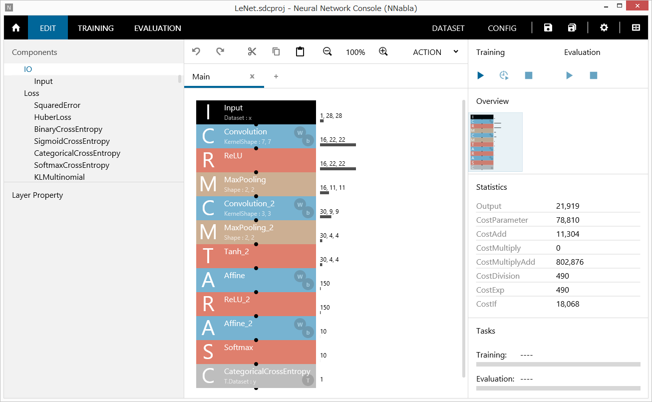
LeNet sample project
Profiling execution
After loading the project, right-click the Run Training button to open a shortcut menu, and click Profile.
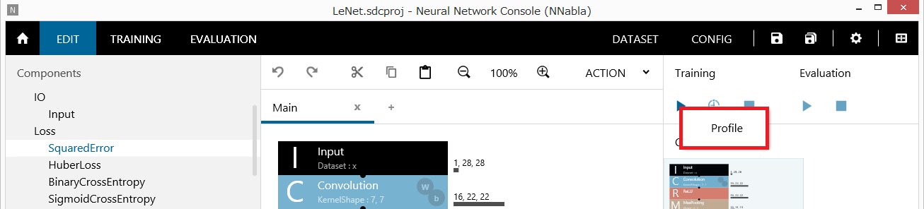
Profiling execution
If training cannot be executed properly, an error will be displayed. If this happens, review the network configuration and dataset settings according to the error message.
When profiling starts properly, the following log is output in place of a training log.
|
load_dataset 2.692669(ms) let_data (x to Input) 0.288460(ms) let_data (y to CategoricalCrossEntropy_T) 0.303508(ms) setup_function (Convolution : Convolution) 0.005436(ms) setup_function (ReLU : ReLU) 0.003144(ms) setup_function (MaxPooling : MaxPooling) 0.003172(ms) setup_function (Convolution_2 : Convolution) 0.003984(ms) setup_function (MaxPooling_2 : MaxPooling) 0.004164(ms) setup_function (Tanh_2 : Tanh) 0.003220(ms) setup_function (Affine : Affine) 0.003720(ms) setup_function (ReLU_2 : ReLU) 0.003057(ms) setup_function (Affine_2 : Affine) 0.003823(ms) setup_function (Softmax : Softmax) 0.002936(ms) setup_function (CategoricalCrossEntropy : CategoricalCrossEntropy) 0.003911(ms) forward_function (Convolution : Convolution) 8.480232(ms) forward_function (ReLU : ReLU : in_place) 2.238630(ms) forward_function (MaxPooling : MaxPooling) 2.542305(ms) forward_function (Convolution_2 : Convolution) 5.676037(ms) forward_function (MaxPooling_2 : MaxPooling) 0.862022(ms) forward_function (Tanh_2 : Tanh) 0.087367(ms) forward_function (Affine : Affine) 0.642076(ms) forward_function (ReLU_2 : ReLU : in_place) 0.072308(ms) forward_function (Affine_2 : Affine) 0.030612(ms) forward_function (Softmax : Softmax) 0.011287(ms) forward_function (CategoricalCrossEntropy : CategoricalCrossEntropy) 0.004772(ms) prepare_backward 0.010244(ms) backward_function (CategoricalCrossEntropy : CategoricalCrossEntropy) 0.007124(ms) backward_function (Softmax : Softmax) 0.007879(ms) backward_function (Affine_2 : Affine) 0.061124(ms) backward_function (ReLU_2 : ReLU : in_place) 0.036198(ms) backward_function (Affine : Affine) 1.232067(ms) backward_function (Tanh_2 : Tanh) 0.015357(ms) backward_function (MaxPooling_2 : MaxPooling) 0.084125(ms) backward_function (Convolution_2 : Convolution) 10.869265(ms) backward_function (MaxPooling : MaxPooling) 0.243760(ms) backward_function (ReLU : ReLU : in_place) 1.690292(ms) backward_function (Convolution : Convolution) 6.254087(ms) forward_all 19.351335(ms) backward_all 21.065874(ms) backward_all(wo param zero_grad) 22.238991(ms) update (Adam) 0.103355(ms) monitor_loss 0.185341(ms) Profile Completed. |
Example of log output of profiling results
Log interpretation
This section describes the output log. All the times indicated in the log are those for processing the number of data samples specified by Mini-batch (in units of milliseconds).
Load dataset
This indicates the time needed to loaded the dataset from storage.
Let data
This indicates the time needed to transfer the loaded dataset to the NNabla engine. The information in parentheses indicates that the substitution source and substitution destination are variable name in the dataset to variable name of NNabla.
Generate data
This does not appear in the previous log, but if the network contained a generator (signal generator), this indicates the time needed to generate the data and substitute it into the Nnabla variable.
Setup function
This indicates the time needed to initialize each layer. The information in parentheses indicates the layer name on Neural Network Console (the Name property value of the layer) : the NNabla class name used in computation. If a GPU (CUDA, cuDNN) is in use, the NNabla class name will include Cuda or CudaCudnn. This allows you to confirm whether the processing of all the layers in the network is being performed on the GPU. Because initialization is performed only once at the start of training, the effect that the value indicated here has on the entire calculation time is negligible.
Forward function
This indicates the time needed in the forward calculation of each layer. Layers that include “: in-place” indicate that the NNabla variable is being shared between input and output to conserve memory usage. Further, by referring to the order in which the forward functions appear in the log, you can confirm the actual order of forward calculations during training.
Prepare backward
This indicates the time needed in the preprocessing of backward calculations of the network.
Backward function
This indicates the time needed in the backward calculation of each layer. The log format is the same as that of forward function.
Forward_all
This indicates the total time needed to perform forward calculation from neural network input to loss function. Because the entire speed is measured separately from the forward function, this may not match the total time displayed for the forward function.
Backward_all
This indicates the total time needed to perform backward calculation from neural network loss function to parameters. wo param zero_grad indicates the time needed to initialize the buffer area for holding the parameter derivatives to zero within the backward calculation.
Weight decay
This does not appear in the previous log, but if weight decay (L2 regularization) is specified in the Optimizer Config, this indicates the time needed to compute the weight decay of all parameters specified to be trained in the network.
Update
This indicates the computation time needed to update all parameters specified to be trained in the network. The information in parentheses indicates the class name of NNabla Solver used to update parameters.
Monitor loss
This indicates the processing time needed to read the output values of the loss function for learning curve monitoring.
Graphing the profiling results
Profiling results can be analyzed in more detail by using the profiling results saved in CSV format in the training result output folder. To open the training result output folder, double-click the training result on the TRAINING tab or right-click to open a shortcut menu, and click Open Result Location.
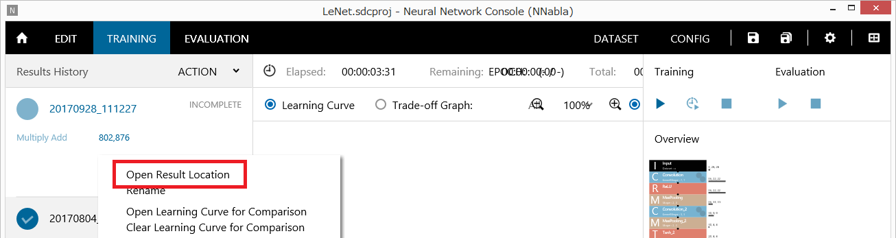
Opening the training result output folder
The profiling results are saved in the file profile.csv in the training result output folder. For example, you can open profile.csv in Excel, and apply conditional formatting to the processing time from Forward function to Backward function to show the processing time graphically.
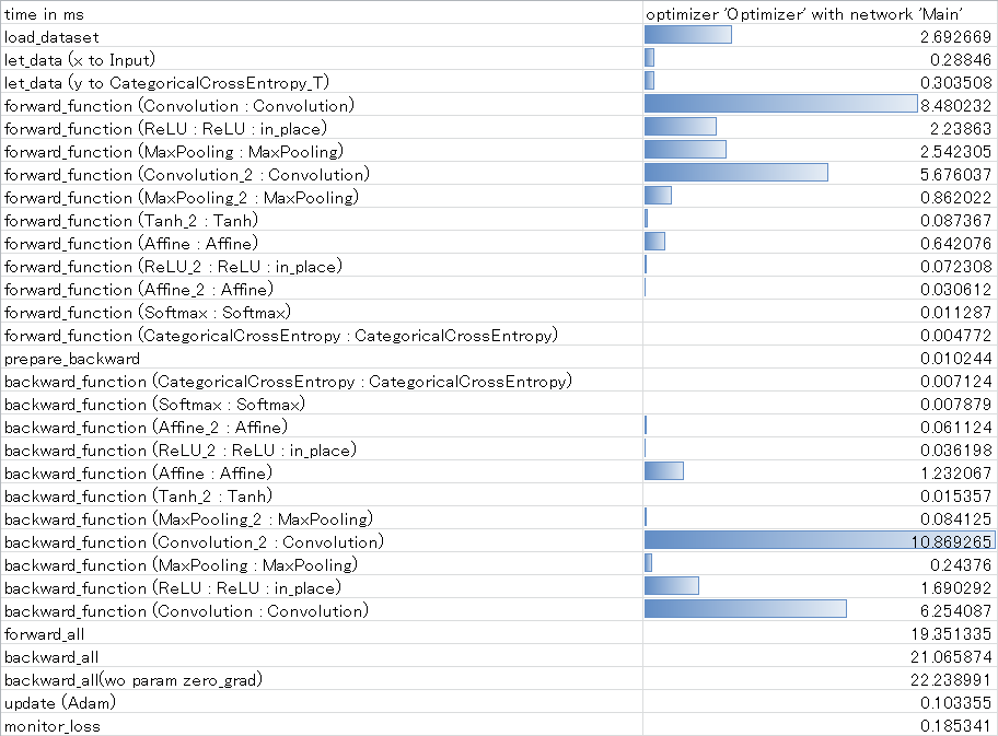
Showing graphically the time needed from Forward to Backward